[ADS-FINAL-PREP] 1. Complexity and Memory
Analyzing complexity and memory usage is the foundation of developing efficient algorithms. This section is dedicated to understanding and evaluating the execution time of algorithms and their impact on memory consumption.
Time Complexity
Time complexity describes how the execution time of an algorithm changes as the input size increases. It is measured in terms of Big O notation (asymptotic complexity).
Main Categories of Time Complexity:
- O(1) – Constant Complexity
- Execution time does not depend on the size of the input data.
- Example: Accessing an array element by index.
- O(log n) – Logarithmic Complexity
- The algorithm reduces the volume of data by half at each step.
- Example: Binary search.
- O(n) – Linear Complexity
- The algorithm iterates through all elements.
- Example: Finding the maximum value in an array.
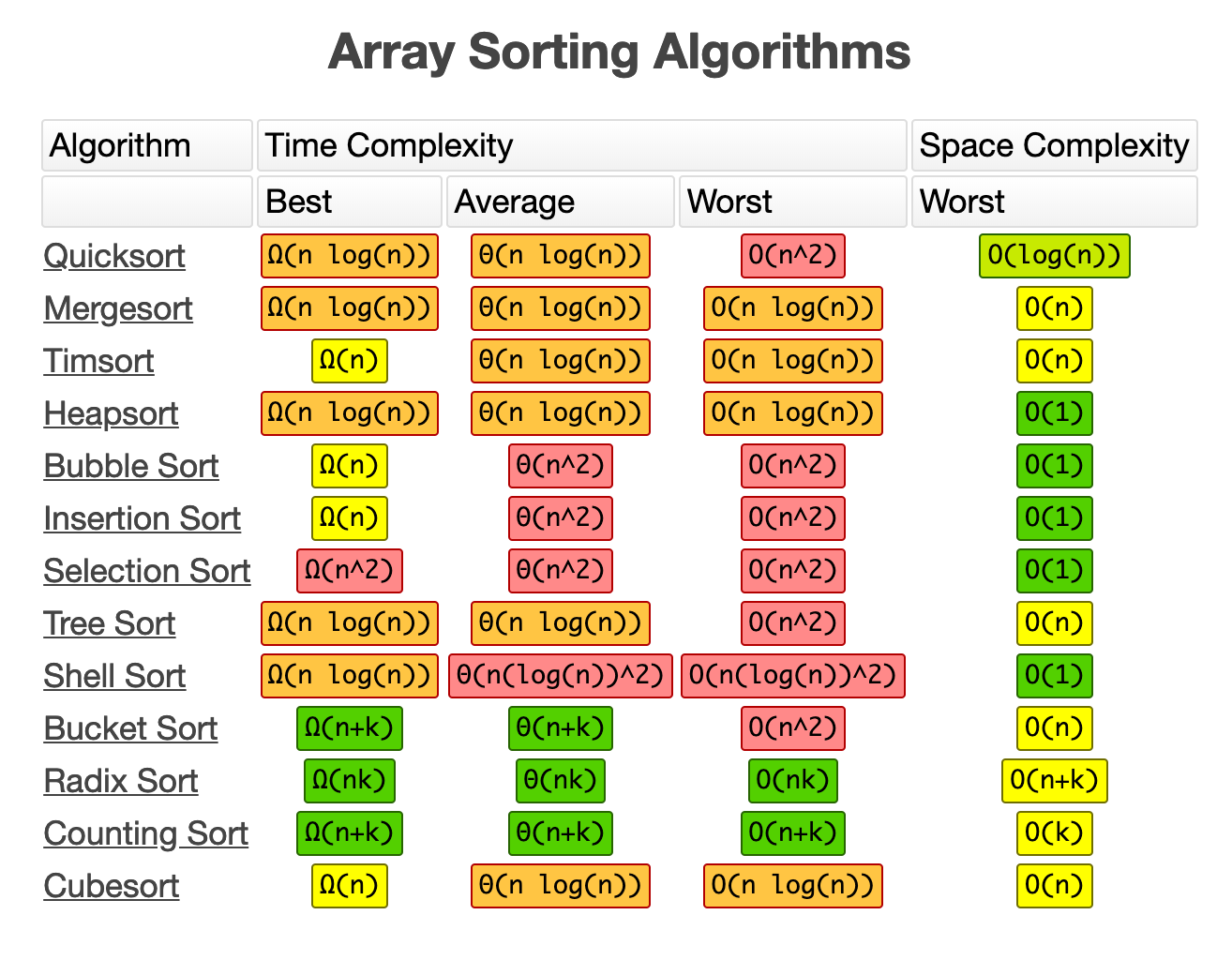
- O(n log n) – Quasilinear Complexity
- Commonly found in sorting algorithms.
- Example: Quick Sort, Merge Sort.
- O(n²) – Quadratic Complexity
- Typical for algorithms that use nested loops.
- Example: Bubble Sort, checking all pairs of elements.
- O(2ⁿ) – Exponential Complexity
- Execution time doubles with each additional input element.
- Example: Solving problems by brute-forcing all combinations (e.g., the Knapsack Problem).
- O(n!) – Factorial Complexity
- Algorithms that iterate through all possible permutations.
- Example: The Travelling Salesperson Problem (in its simplest brute-force approach).
Why Is This Important?
- Optimization: Complexity allows you to choose the best algorithm for a task, especially when dealing with large datasets.
- Comparison: For example, Bubble Sort O(n²) is far less efficient than Merge Sort O(n log n).
- Real-world Applications: Algorithms for large databases, web services, and machine learning depend heavily on time and space complexity.
If you noticed a mistake or copyright issues, please contact: lebroskiofficial@proton.me